Building a Convolutional Neural Network(CNN) From Scratch (WIP)

Problem Formulation

Description

Our goal is to build a Convolutional Neural Network(CNN) from scratch to classify handwritten digits (0–9) from the MNIST dataset. We will design a neural network architecture that takes 28x28 pixel grayscale image and outputs a probability distribution over the 10 classes.

We will train and implement this network from scratch without using any built in pytorch functionalities, that is building our own dataloading functionality and forward and backward propagation for each module.

Mathematical Formulation

The architecture that follows the input image to the final layer is detailed in Architecture Details. Mathamtically, for a given input image (x), we want to produce a probability vector (p) over the classes. We use the softmax function after the final layer, where (z) is the output of the dense layer before softmax. Given that we have (z),

The softmax probability for class ( i ) is given by:

\[p_i = \frac{e^{z_i}}{\sum_{j=1}^{10} e^{z_j}}\]

The predicted class $( \hat{y} )$ is computed as the index of the maximum probability:

\[\hat{y} = \arg\max_i p_i\]

The cross-entropy loss $( L )$ is defined as:

\[L = -\sum_{i=1}^{10} t_i \log(p_i)\]

$( t_i )$ is one-hot encoded, only one term in the summation contributes.

MNIST Dataset

The MNIST dataset consists of:

• 60,000 training images
• 10,000 testing images

Figure 1: An example from the MNIST dataset.

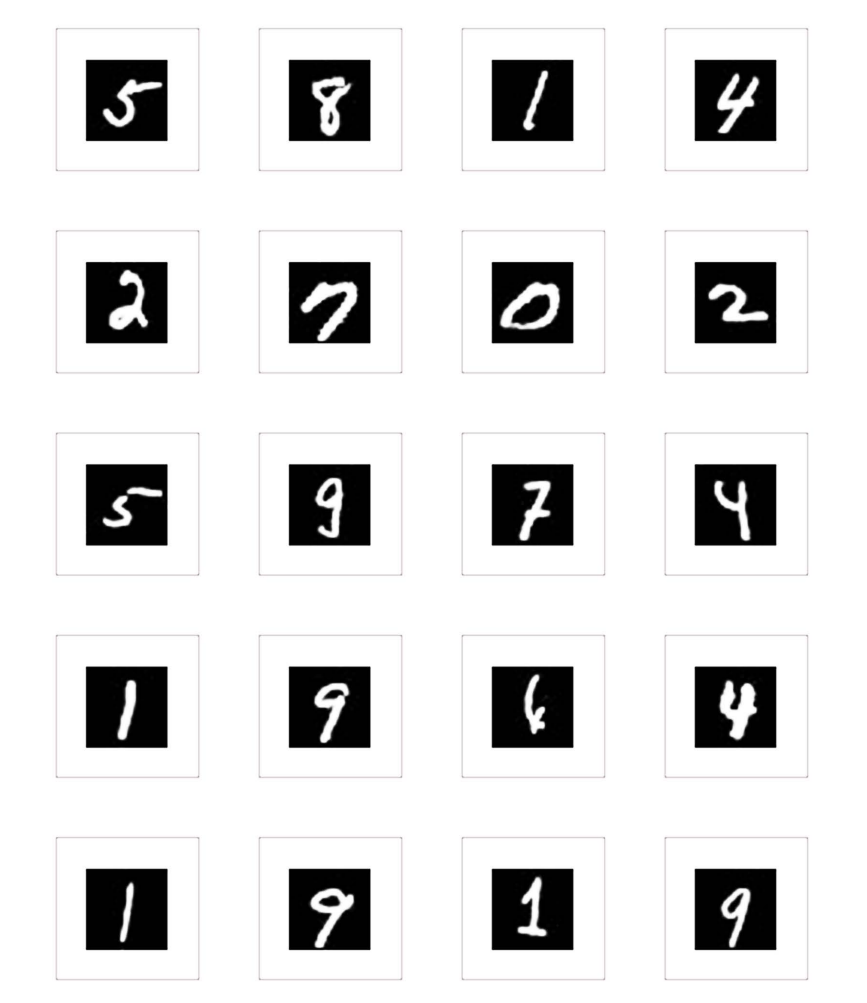
Each image is normalized to [0,1] and we one-hot encode the labels for training.

For example, the digit ‘3’ would be encoded as ([0,0,0,1,0,0,0,0,0,0]).

Architecture Details

Overview

Figure 2: This is the architecture that we will use in this implementation.

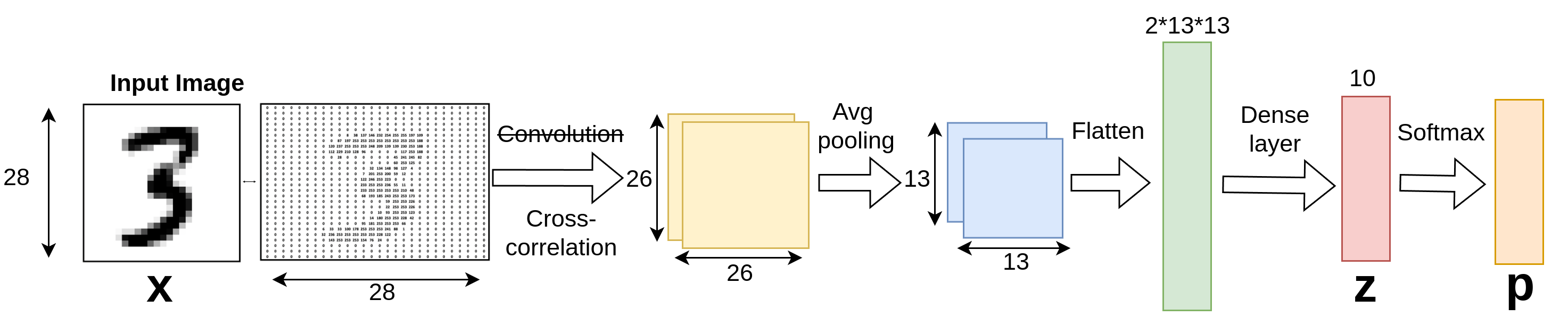
This architecture represents a simple Convolutional Neural Network (CNN) for digit classification using the MNIST dataset. The network begins with an input image of size \((28 \times 28)\), which undergoes the following stages:

1. Cross-Correlation (also known as Convolution in Deep Learning): The input is processed through a cross-correlation layer that applies filters, resulting in a feature map of size \((26 \times 26)\).
2. Average Pooling: The feature map is downsampled using average pooling, reducing its size to \((13 \times 13)\).
3. Flattening: The downsampled feature map is flattened into a one-dimensional vector of size \((2 \times 13 \times 13)\).
4. Dense Layer: The flattened vector is passed through a fully connected (dense) layer to produce a vector z of size 10.
5. Softmax Layer: Finally, a softmax activation on the vector z produces the output probabilities p for each of the 10 digit classes.

1. Convolutional (or more like Cross-correlation) Layer

It is important to clarify that cross-correlation$(\star)$ is not the same as convolution$(\ast)$. In fact, what we usually refer to as convolution in neural networks is actually implemented using cross-correlation. This distinction is important, as we will design functions later when implementing these operations. For a more detailed explanation of these operations, read more here.

The mathematical relationship between convolution and cross-correlation can be expressed as:

\[I\star K = I * \text{rot}_{180}(K)\]

Here:

• \(I\) is the input, \(K\) is the kernel, \(\text{rot}_{180}(K)\) represents the 180-degree rotation of the kernel \(K\).

Forward Propagation

In this architecture, forward propagation is performed by applying the kernels (filters) to the input image using cross-correlation and adding the respective biases as visualized in Figure 4 for $Y^1_{11}$. Similarly, sliding the kernel over the input image will give us $Y1$.

Figure 4: Visualization of spplying two $ 3\times 3$ filters for a input image of $28 \times 28$. Correlation operation to compute $Y^1_{11}$ is highlighted by red. Sliding the kernel $K1$ over the input image will give us $Y1$, and $K2$ likewise $Y2$.

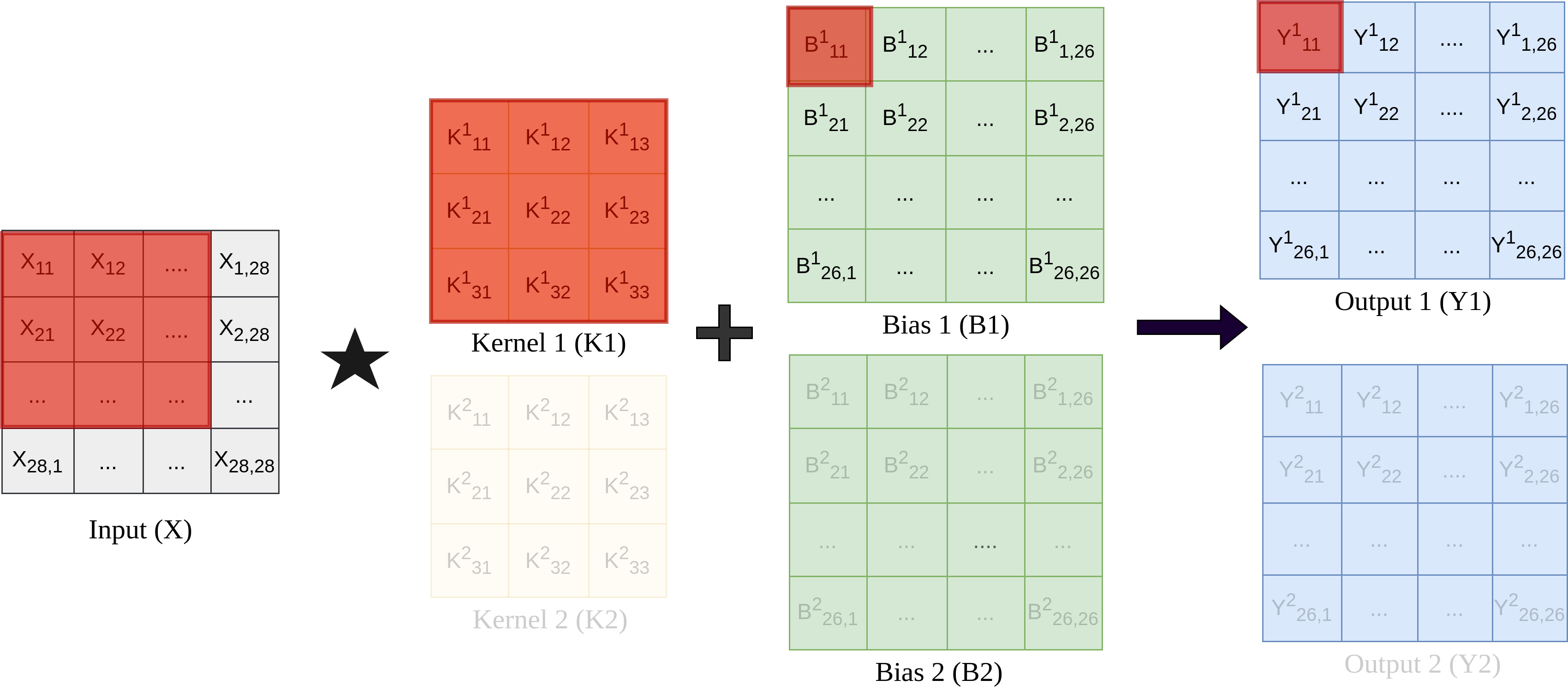
NOTE

This can be generalized: For example, an RGB input with depth 3 and 10 kernels would produce 10 feature maps. The kernel depth matches the input depth, and biases are added channel-wise.

As shown in figure 4, for the given setup with two kernels, in the matrix form, the output feature maps are computed:

$$ Y^1 = B^1 + X \star K^1 $$

\[Y^2 = B^2 + X \star K^2\]

In general (kernel size = n),

\[Y^n = B^n + X \star K^n\]

For each output element of kernel operation, the value is calculated by summing the element-wise multiplication of the kernel and the corresponding area of the input image. The formula for this operation is:

\[Y_{i,j} =Y[i, j] = \sum_{m=0}^{M-1} \sum_{n=0}^{N-1} X[i+m, j+n] \cdot K[m, n] + B_{i,j}\]

In our case, we use 2 filters (kernels) of size \(3 \times 3\) (m=n=3) and perform valid cross-correlation on the input image, followed by a sigmoid activation function to obtain outputs of shape \(26 \times 26\).

The formula for calculating the output size is:

\[O = \frac{I - K + 2P}{S} + 1\]

(Substituting: \(I = 28\), \(K = 3\), \(P = 0\), \(S = 1\))

\[O = \frac{28 - 3 + 2(0)}{1} + 1 = 26\]

Thus, the output feature map has dimensions \(26 \times 26\).

Backpropagation

In a convolutional layer, the objective during backpropagation is to compute the following:

1. Gradients with Respect to Kernels $(\frac{\partial L}{\partial K} )$: To update the kernel weights.
2. Gradients with Respect to Biases $( \frac{\partial L}{\partial B} )$: To update the bias terms.
3. Gradients with Respect to the Input $(\frac{\partial L}{\partial X} )$: To propagate the error back to the previous layer.

We are given the gradient of the loss with respect to the output of this layer $(\frac{\partial L}{\partial Y})$, referred to as the output gradient. Using this, we calculate the necessary gradients for kernel updates, bias updates, and input gradients.

1. Gradients with Respect to Kernels $(\frac{\partial L}{\partial K})$:

To update the kernel weights, we compute the gradient of the loss with respect to each kernel element. This is calculated using a valid correlation between the input X and the output gradient $( \frac{\partial L}{\partial Y} )$.

\[\frac{\partial L}{\partial K^i} = X \star \frac{\partial L}{\partial Y^i}\]

For a given kernel (K), this is computed as:

\[\frac{\partial L}{\partial K_{m,n}}= \frac{\partial L}{\partial K}[m, n] = \sum_{i=0}^{O-1} \sum_{j=0}^{O-1} X[i+m, j+n] \cdot \frac{\partial L}{\partial Y}[i, j]\]

2. Gradients with Respect to Biases $( \frac{\partial L}{\partial B} )$:

Bias gradients are simply computed by summing the output gradients over all spatial positions:

\[\frac{\partial L}{\partial B^i} = \frac{\partial L}{\partial Y^i}\]

3. Gradients with Respect to the Input $( \frac{\partial L}{\partial X} )$:

To propagate the error backward to the previous layer, we compute the gradient of the loss with respect to the input. This involves performing a full convolution between the output gradient $( \frac{\partial L}{\partial Y} )$ and the kernel (K):

\[\frac{\partial L}{\partial X} = \sum_{i=1}^{n} \frac{\partial L}{\partial Y^i} *_{\text{full}} K^i\] \[\frac{\partial L}{\partial X_{i,j}} =\frac{\partial L}{\partial X}[i, j] = \sum_{m=0}^{M-1} \sum_{n=0}^{N-1} \frac{\partial L}{\partial Y}[i-m, j-n] \cdot K_{\text{flipped}}[m, n]\]

This operation results in a gradient for the input that matches its original dimensions, allowing error propagation backward through the network.

Code

tba

---

2. Sigmoid Activation

The sigmoid activation function introduces non-linearity into the network, and we use this activation on the convolutional layer.

Forward Propagation

In forward propagation, the sigmoid activation function computes the output as:

\[\sigma(x) = \frac{1}{1 + e^{-x}}\]

Backpropagation

\[\sigma'(x) = \sigma(x) \cdot (1 - \sigma(x))\]

Code

tba

---

3. Average Pooling

The average_pooling class implements an average pooling layer, which is applied after the convolutional layer. This layer reduces the spatial dimensions of the input while preserving essential information, making it computationally efficient and robust to small transformations.

Forward Propagation

During the forward pass, the layer applies average pooling to the input. This involves iterating over the input’s spatial dimensions, selecting windows of size pool_size, and computing the average value for each window.

The operation can be described mathematically as:

\[Y_{ij} = \frac{1}{N} \sum_{m,n} X_{(i+m)(j+n)}\]

Backpropagation

In the backward pass, gradients are propagated back to the input by equally distributing the gradient of the output across the corresponding input elements in the pooling window. The backpropagation is described as:

\[dX_{(i+m)(j+n)} += \frac{dY_{ij}}{N}\]

Code

tba

4. Flatten Layer

Flatten layer converts multi-dimensional data (e.g., feature maps) into a one-dimensional vector. This transformation is necessary to connect the convolutional or pooling layers to fully connected (dense) layers.

Code

tba

5. Dense Layer

Forward Pass:

\(\text{y} = W \cdot x + b\)

Backpropagation for Dense Layer

1. Gradients with Respect to Weights :

   \[\frac{\partial L}{\partial W} = x^T \cdot \frac{\partial L}{\partial Y}\]

2. Gradients with Respect to Biases :

   \[\frac{\partial L}{\partial b} = \frac{\partial L}{\partial Y}\]

3. Gradients with Respect to the Input :

   \[\frac{\partial L}{\partial x} = \frac{\partial L}{\partial Y} \cdot W^T\]

Code

tba

6. Softmax

Code

tba